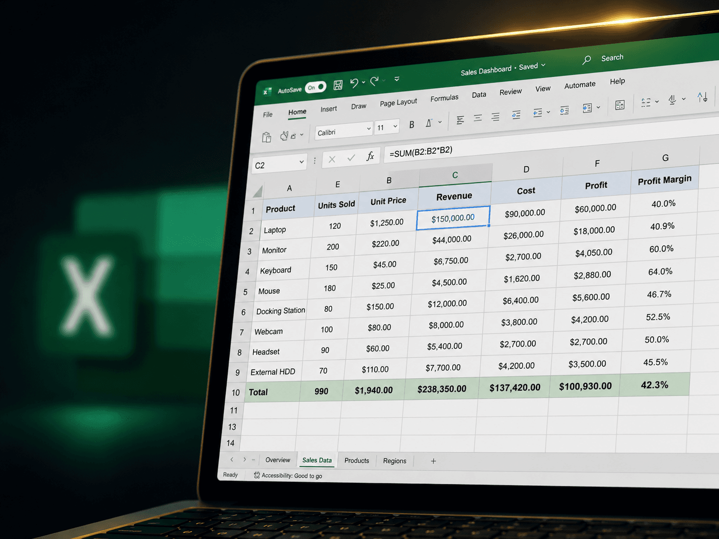
Professional Excel Tips and Tricks Every User Should Know

Excel rewards people who know its shortcuts. The difference between someone who fumbles through ribbons and someone who moves through a workbook in seconds usually comes down to a handful of habits, not advanced training. Here are the ones worth actually memorizing.

Navigation shortcuts that save the most time

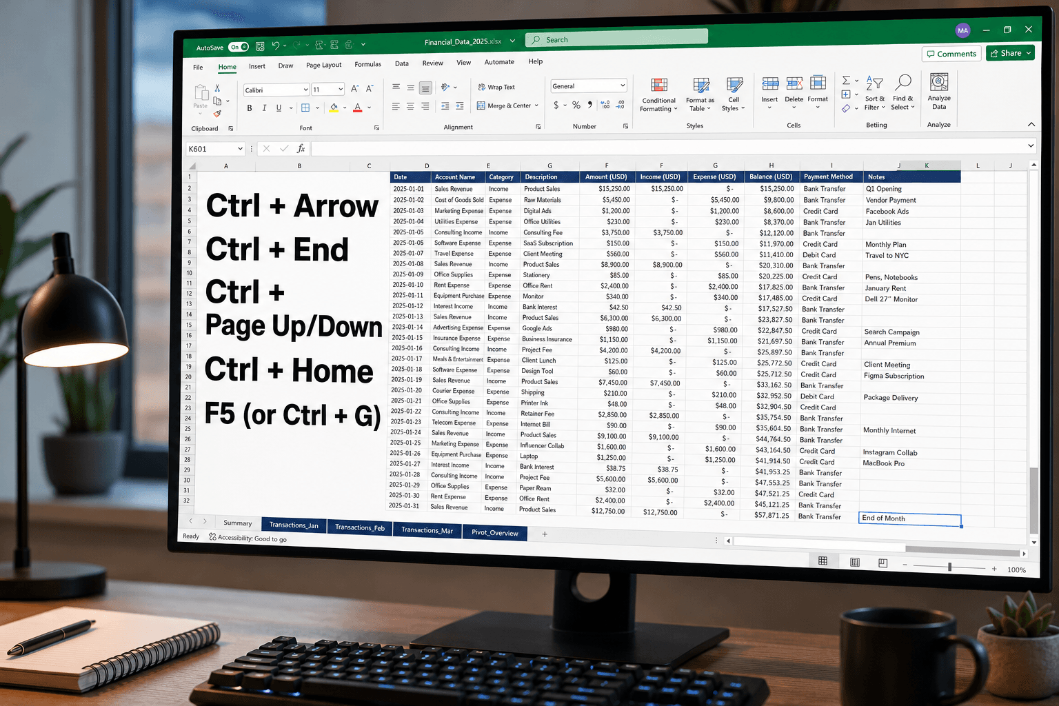
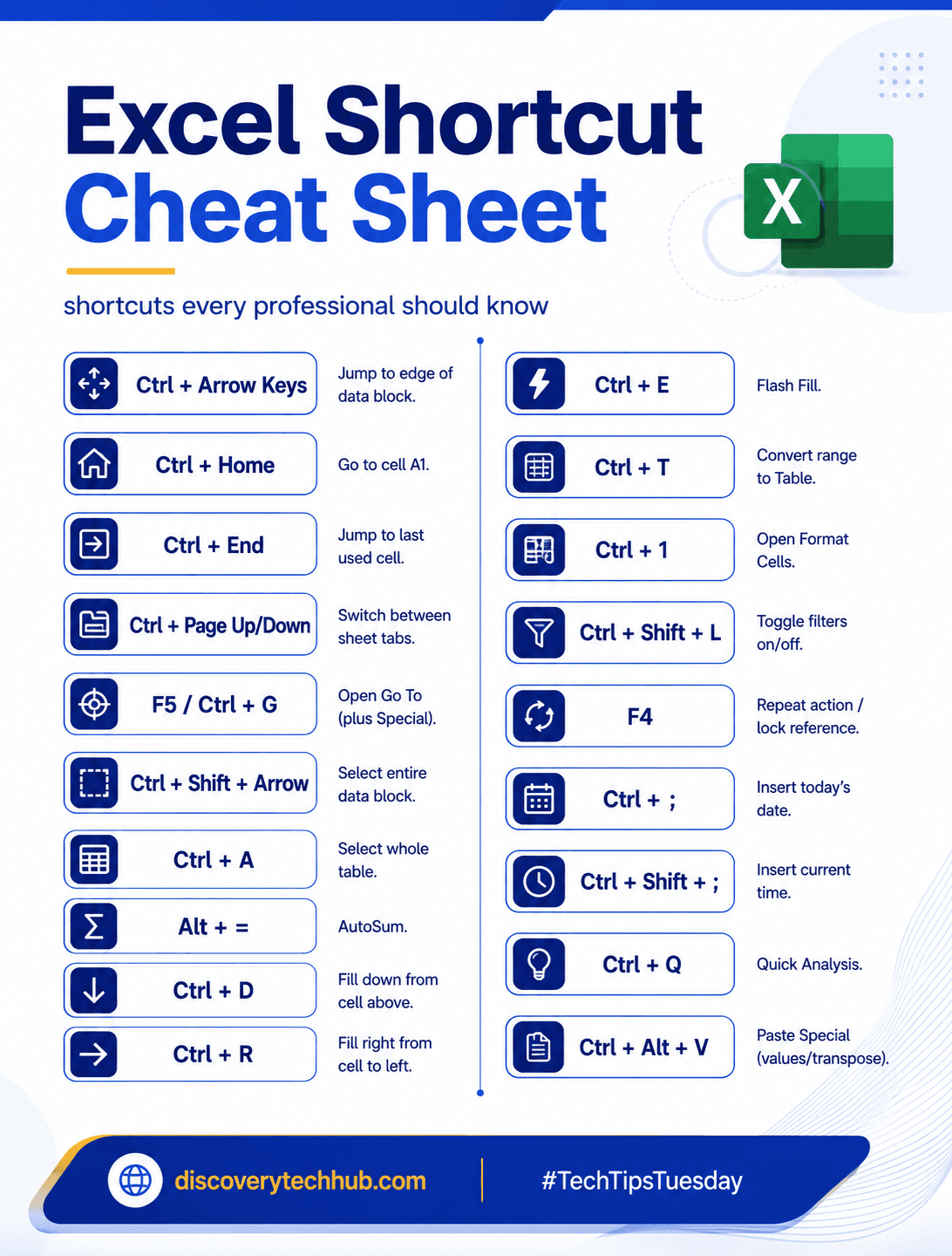
Ctrl + Arrow keys jump to the edge of a data block instantly, instead of scrolling. Ctrl + Home takes you to cell A1 from anywhere in a sheet, and Ctrl + End jumps to the last used cell, which is handy for spotting stray formatting far outside your actual data. Ctrl + Page Up/Down switches between sheet tabs without touching the mouse. F5 (or Ctrl + G) opens Go To, which becomes powerful once combined with Special (Go To Special lets you select only blanks, only formulas, or only visible cells in a filtered range).

Selecting and entering data faster

Ctrl + Shift + Arrow selects an entire block of data in one move, and Ctrl + A selects the whole table when your cursor sits inside it. Alt + = triggers AutoSum instantly. Ctrl + D fills a formula or value down from the cell above, and Ctrl + R fills right, both far faster than dragging a fill handle. Double-clicking the fill handle itself auto-extends a formula down to match an adjacent column's length, which is one of the most underused tricks in the program.

Flash Fill: the trick most people never discover

Flash Fill (Ctrl + E) detects a pattern from an example you type and applies it to the rest of the column automatically. Type a full name split into first and last name once, and Flash Fill will split every other row the same way, no formula required. It works for reformatting dates, extracting parts of an email address, combining columns, or cleaning up inconsistent text.

Formulas every professional should know

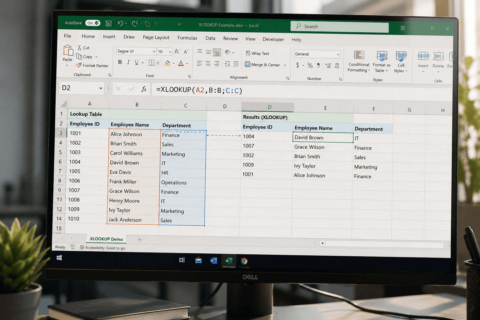
XLOOKUP has replaced VLOOKUP as the modern standard. It searches in any direction, handles missing matches cleanly, and doesn't break when a column is inserted:

=XLOOKUP(lookup_value, lookup_array, return_array)

INDEX/MATCH is still worth knowing for older files or more complex lookups:

=INDEX(return_range, MATCH(lookup_value, lookup_range, 0))

IFERROR wraps around any formula to replace errors with a clean value instead of #N/A or #DIV/0!:

=IFERROR(formula, "Not found")

SUMIFS and COUNTIFS let you total or count data based on multiple conditions at once, which covers most reporting needs without a pivot table:

=SUMIFS(sum_range, criteria_range1, criteria1, criteria_range2, criteria2)

TEXTJOIN combines multiple cells into one string with a chosen delimiter, ignoring blanks automatically, which is far cleaner than chaining CONCATENATE.

Named ranges instead of cell references

Selecting a range and typing a name into the Name Box (top-left, next to the formula bar) lets you reference it by name anywhere in the workbook, for example =SUM(Revenue) instead of =SUM(B2:B50). This makes formulas easier to read and far easier to audit later.

Formatting that actually communicates

Conditional formatting (Home → Conditional Formatting) highlights values automatically based on rules, turning a plain table into something a manager can scan in seconds. Custom number formats let you display numbers as thousands, percentages, or with units without changing the underlying value, using the Format Cells dialog (Ctrl + 1). Ctrl + 1 is worth memorizing on its own, since it opens the full formatting menu instantly.

Tables, not ranges

Turning a data range into an actual Table (Ctrl + T) gives you automatic formatting, structured references in formulas, and columns that expand automatically as new rows are added. Any formula referencing a table column keeps working even after rows are inserted or deleted, which plain ranges don't handle well.

PivotTables without the fear

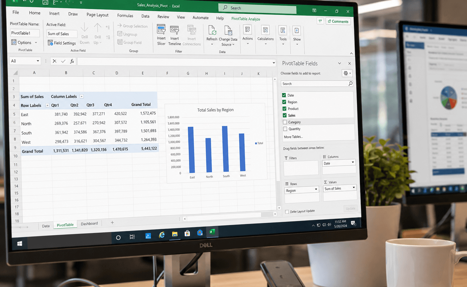
A PivotTable summarizes thousands of rows into a clean report in a few drags. Select your data, go to Insert → PivotTable, then drag fields into Rows, Columns, and Values. Right-clicking a value field and choosing "Show Values As → % of Total" turns raw numbers into a quick share-of-total breakdown without writing a single formula.

Data validation to prevent bad input

Data → Data Validation lets you restrict a cell to a dropdown list, a date range, or a whole number within limits. This is the single best way to stop shared workbooks from filling up with typos and inconsistent entries.

Freeze Panes for long sheets

View → Freeze Panes keeps header rows and label columns visible while scrolling through long datasets, which matters the moment a sheet grows past one screen.

Quick Analysis and Paste Special

Selecting a range and clicking the small Quick Analysis icon (or Ctrl + Q) gives instant chart, total, and formatting suggestions. Paste Special (Ctrl + Alt + V) lets you paste only values, only formulas, or only formatting, and its "Transpose" option flips rows into columns in one click, no manual retyping required.

Keyboard shortcuts worth memorizing today

Ctrl + T (table), Ctrl + 1 (format cells), Ctrl + E (flash fill), Ctrl + Shift + L (toggle filters), F4 (repeat last action, and also toggles absolute references while editing a formula), Ctrl + ; (insert today's date), and Ctrl + Shift + ; (insert current time).

The habit that matters more than any single trick

None of these tools matter much on their own. What separates a confident Excel user is reaching for the keyboard instead of the mouse by default, and knowing which of these dozen tools fits a given problem before starting to build a formula. Pick three from this list you don't currently use, and build them into your next workbook. That's usually enough to notice a real difference in speed within a week.